
Revisiting Deep Learning: AlexNet & ResNet
From depth to skip connections: what AlexNet and ResNet taught us

AlexNet: A deep convolutional network that gave rise to the modern deep learning. It introduces many key ideas such as ReLU activations instead of tanh/sigmoid, multi-GPU training, dropout for regularization, and overlapping pooling.
ResNet: With increasing depth, a notorious problem of vanishing/exploding gradients was observed leading to accuracy getting saturated eventually degrading. It introduced residual blocks, built around skip connections that provide an alternate path for gradient flow. By enabling the network to learn identity mappings, residual connections ensure that deeper layers do not perform worse than shallower ones.
Code is available on github: Code
AlexNet Architecture - Key Features
ReLU Nonlinearity
Traditional nonlinear activation function like tanh/sigmoid suffer from vanishing gradients when neurons saturate. Also exponential function is a bit expensive
Increase the cost and is slow to train
ReLU addressed these issues by providing a non-saturating, piecewise linear activation that is computationally cheap and enables faster, more stable optimization
\(\mathrm{ReLU}(x) = \max(0, x) \)
Local Response Normalization
Biologically inspired mechanism that encourages competition among neurons at the same spatial location across neighboring channels, promoting sparse and locally normalized activations.
For an activation aix,y at spatial location (x,y)(x,y) and channel index ii, the normalized output bix,y
The normalization is performed across channels, not spatially
summation runs over nnn adjacent channels at the same spatial location
N is the total number of channels (feature maps) in the layer
This introduces local competition among nearby feature maps
In AlexNet, LRN uses k = 2, α = 1e-4, β=0.75, and normalizes over n = 5 neighbouring channels.
Why LRN is used?
Although ReLU activations are non-saturating and do not strictly require normalization, LRN was used in AlexNet as a cross-channel normalization mechanism that encouraged local competition, improved generalization, and reduced overfitting in early deep CNNs
In modern times, LRN is replaced by BatchNorm[3]
BatchNorm:
Normalizes activations using batch-wise mean and variance
Stabilizes gradients by reducing internal covariate shift
Accelerates convergence and allows higher learning rates
Learns scale and shift parameters (γ,β)
LRN:
Normalizes activations across neighboring channels at the same spatial location
Does not explicitly stabilize gradients
Introduces additional computation
Relies on hand-tuned hyperparameters (k,α,β,n)
Provides limited regularization compared to BatchNorm
Compute-inefficient on modern hardware:
Requires channel-wise reductions
Leads to poor GPU utilization
Is memory-bandwidth heavy
Poor fit for modern accelerators, lacking efficient fused implementations
Overlapping pooling
Traditional pooling typically uses:
kernel size (k) = stride (s) → non-overlapping regions
e.g., 2×2 pooling with stride 2
AlexNet instead uses:
Max pooling
Kernel size: k=3×3
Stride: s=2
Because s < k, adjacent pooling windows overlap.
The authors observed the following:
Reduces error rates compared to non-overlapping pooling
Acts as a regularizer
Slightly increases computation, but with measurable gains
Reducing overfitting
Data Augmentation
Random cropping
Preprocessing
Original ImageNet images were rescaled so the shorter side = 256
Aspect ratio preserved
During training
Random 224 × 224 crops were sampled from the resized image
During testing
Center crop was used
Why it helps
Translation invariance
Forces robustness to object position
Multiplies dataset size implicitly
Horizontal flipping
Each crop was randomly mirrored
Doubles the effective dataset size
Why it helps
Objects are usually left–right symmetric
Safe augmentation (label preserved)
Very cheap computationally
PCA-based color augmentation (important & non-obvious)
The technique perturbs image colors in a statistically grounded way, rather than using arbitrary jitter.
This was novel at the time.
What they did
Compute PCA on RGB values (offline)
Collect all RGB pixel values from the ImageNet training set
Treat each pixel as a 3D vector [R,G,B]
Perform PCA on this distribution
This yields:
Eigenvectors P ∈ ℝ3X3 → principal directions of color variation
Eigenvalues Λ = [λ1,λ2,λ3] → magnitude of variation along each direction
For each training image, modify every pixel as:
Where:
I(x,y) is the original RGB pixel
α is a random coefficient
⊙: element-wise multiplication
The same RGB offset is added to every pixel
Why it helps
Simulates lighting changes
Preserves structure while altering color statistics
Improves color invariance
Dropout
Where dropout was applied
Only in fully connected layers
FC6
FC7
Not used in convolutional layers
Why dropout was necessary in AlexNet
1. Massive parameterization
~60 million parameters
Majority in FC layers
Without dropout:
Model memorized ImageNet
Training error decreased rapidly
Validation error shot up → severe overfitting
2. Prevents co-adaptation
Dropout forces neurons to:
Work independently
Learn redundant representations
Avoid brittle feature dependencies
This was crucial before BatchNorm existed.
ResNet18 Architecture - Key Features
Residual Learning(The Big Idea)
Prior to this, training deeper networks often performed worse than their shallower counterparts. When deeper networks start to converge, a degradation problem was observed: with network depth increasing, accuracy gets saturated and then degrades rapidly. Such degradation is not caused by overfitting, and adding more layers to a suitably deep model leads to higher training error.
Residual learning was introduce to optimize such systems.
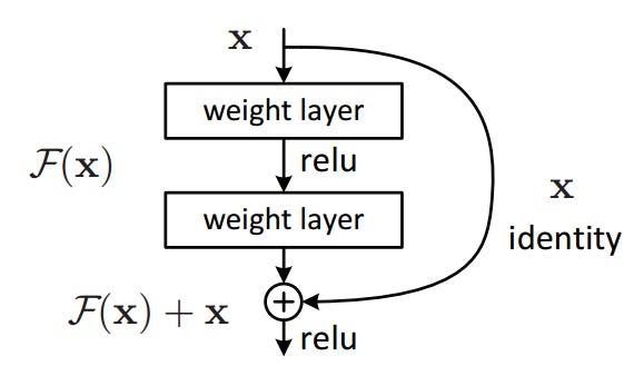
Let’s consider H(x) where x is the input, that a neural network is trying to learn.
Instead of learning H(x) directly, the network leans a residual function F(x) = H(x) - x.
So the original function becomes H(x) = F(x) + x
In short, the network learns change relative to the input instead of relearning the entire transformation.
In practice,
Idea is implemented using skip(shortcut) connections.
An typical of a residual block[2] is shown below, consisting of few stacked layers (e.g., Conv → BN → ReLU), shortcut connection that bypasses these layers, element-wise addition of the input and the block’s output.
These skip connections are:
Parameter-free
Identity mappings
Simple additions
Why is this useful?
Solves the degradation problem
As networks get deeper:
Training error increases after a point (even without overfitting)
Gradients become weak or unstable
Residual connections allow gradients to flow directly through the network, bypassing multiple nonlinear layers. This stabilizes optimization and makes very deep models trainable.
Identity mapping is easy to learn
Bottleneck Architecture
For very deep networks (50+ layers), ResNet introduced the bottleneck block:
1×1 conv → 3×3 conv → 1×1 conv
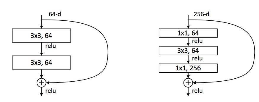
Why it matters?
1×1 convolutions reduce and restore channel dimensions
Significantly lowers:
Parameters
FLOPs
Makes 100+ layer networks computationally feasible