Revisiting DeepLearning: DenseNet, MobileNet, EfficientNet

From feature reuse to efficiency-driven design

In the previous post, I explored how AlexNet popularized deep CNNs and how ResNet solved the vanishing gradient problem using residual connection. However, depth alone was not the end and in this blog will focus on architectures which introduced different kind of efficiency strategies.

DenseNet, MobileNet, EfficientNet each rethink CNN design by optimizing different aspect of efficiency.

• DenseNet → efficiency via feature reuse

• MobileNet → efficiency via computation reduction

• EfficientNet → efficiency via systematic scaling

I will focus on the Image Classification task in this blog.

Code can be found at: GitHub Link

DenseNet

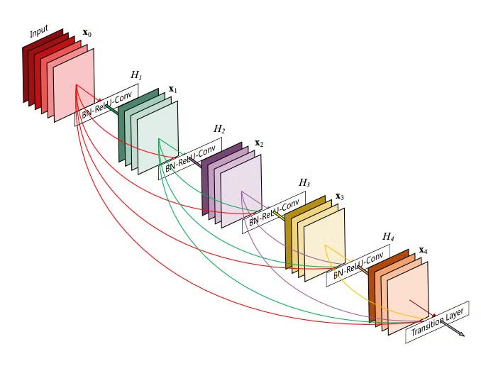
DenseNet(Densely Connected Convolutional Network) changed how neural network layers communicate. Instead of each layer only receiving input from the previous layer, every layer has direct access to all previous feature maps. This dense connectivity allows information and gradients to flow easily throughout the network.

DenseBlock concept

For a dense block:

• Operation Sequence: Each layer applies ReLU, then 2D convolution, and then concatenates the output to previous features.

• Mathematically:

  • x_l = H_l([x₀,x₁, …, x_l-1])

    • where H_l(.) is the convolution and activation operations.

Padding to preserve Spatial Dimensions

• padding = (k - 1) / 2, where k is the kernel size

Dense Block Growth

• Each layer within a Dense Block produces ‘growth_rate’ feature maps.

• After L layers, total_channels = input_channels + L * growth_rate

• growth_rate: critical hyperparameter as this controlled growth keeps the network relatively parameter-efficient.

For example, as being observed from Fig.1, for L layers, there are L*(L + 1) / 2 direct connections. For each layer, feature maps of all preceding layers are used as input and its own feature map used in all subsequent layers. That’s it.

Fig.1: 5-layer dense block with a growth rate of k = 4^[1]

Defining Design choice: feature concatenation instead of summation, unlike in ResNet where layers are connected via additive skip connections. DenseNet preserves feature maps explicitly, avoiding information loss and enabling effective feature reuse.

Key Characteristics:

• Alleviate vanishing gradient problem through multiple short gradient paths

• Strengthen feature propagation across layers

• Encourage feature reuse, reducing redundancy

• Parameter reduction: eliminates the need to learn redundant features

While DenseNet improved parameter efficiency and gradient flow, its memory cost made it less suitable for resource-constrained environments.

MobileNet

For many real-world applications, however, the primary constraint is not training stability or parameter count, but computational cost and inference latency.

MobileNet was introduced to address this challenge. MobileNet redesigns the convolution operation itself to drastically reduce computation.

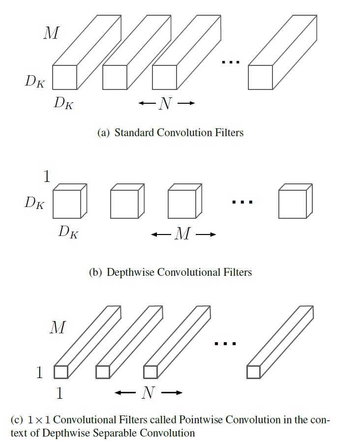
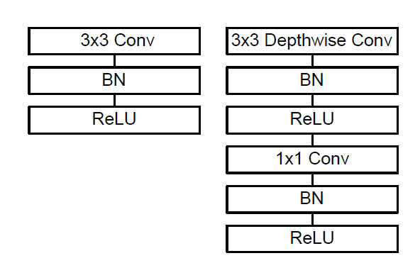
DepthWise Separable Convolution

Core idea is to factorize a standard convolution into two operations:

• Depthwise Convolution: applies a single convolutional filter to each input channel independently.

• Poistwise Convolution(1x1): combines the outputs across channels

Consider an input feature map F of shape D_F x D_F x M where:

• D_F : spatial resolution (height and width)

• M : number of input channels

Goal: Produce an output feature map G of shape D_G x D_G x N, where:

• N: number of output channels

Standard Convolution

In a standard convolutional layer, using kernel of size D_K x D_K x M x N

• Each output channel is computed by convolving across all input channels, tightly coupling spatial filtering and channel mixing.

Total Computational Cost = D_K . D_K . M . N . D_F . D_F

Depthwise Separable Convolution

1. Depthwise Convolution

   • Applies one filter D_K x D_K per input channel

   • No mixing across channels

   • Computational cost = D_K . D_K . M . D_F . D_F

2. Pointwise Convolution (1x1)

   • Uses 1 x 1 convolutions to combine channel information

   • Maps M input channels to N output channels

   • Computational cost = M . N . D_F . D_F

Total computational cost = D_K . D_K . M . D_F . D_F + M . N . D_F . D_F

Net reduction = (1 / N) + (1 / D²_K )

For typical values(D_K = 3, large N):

• Computation reduce 8-9x

• Accuracy degradation is relatively small

Fig.2: The standard convolutional filters in (a) are replaced by two layers: depthwise convolution in (b) and pointwise convolution in (c) to build a depthwise separable filter^[2]

Fig.3: Left: Standard convolutional layer with batchnorm and ReLU. Right: Depthwise Separable convolutions with Depthwise and Pointwise layers followed by batchnorm and ReLU^[2]

Width and Resolution Multipliers

MobileNet introduces two simple hyperparameters to control the trade-off between accuracy and efficiency:

• Width multiplier (α): scales the number of channels in each layer

• Resolution multiplier (ρ): scales the input image resolution

The above two hyperparameters can be adjusted to different hardware and latency constraints without redesigning the architecture.

Key Characteristics

• Drastically reduced computation via depthwise separable convolutions

• Lightweight architecture suitable for mobile and embedded devices

• Flexible accuracy–latency trade-off through width and resolution scaling

• Fast inference under tight resource constraints

Subsequent versions of MobileNet refined this lightweight design without changing its core principle(Detailed discussion is beyond the scope of this blog)

• MobileNetV2 introduced inverted residual blocks with linear bottlenecks to improve information flow and training stability

• MobileNetV3 incorporated lightweight attention mechanisms, hardware-friendly activations, and neural architecture search to further optimize accuracy–latency trade-offs.

While MobileNet and the subsequent variants focused on optimizing models for resource-constrained systems, the question of how to systematically scale networks across different compute regimes needs to be explored.

EfficientNet

Increasing model capacity is a common way to improve accuracy, but naïvely scaling a network by only increasing depth, width, or input resolution often leads to diminishing returns.

EfficientNet introduces a systematic scaling strategy, called compound scaling, which jointly scales network depth, width, and resolution in a balanced manner. EfficientNets are designed to get better accuracy with far fewer parameters and FLOPs than prior models (ResNet, DenseNet, etc.).

Core Idea: Compound Scaling

Instead of scaling only depth or width or resolution, EfficientNet scales all three together in a principled way.

Let:

• depth = d, width = w, resolution = r

Before EfficientNets

1. Only increase depth

   • Add more layers

   • Problems: vanishing gradients, diminishing returns

   • E.g.: ResNet-1000 has similar accuracy as ResNet-101 even though it has much more layers.

2. Only increase width

   • Add more channels

   • Problems: memory-heavy, inefficient use of FLOPs

3. Only increase resolution

   • Use bigger images

   • Problems: computation explodes

Scaling up any dimension of network width, depth, or resolution improves accuracy, but the accuracy gain diminishes for bigger models.

Depth, width, and resolution should be scaled together, not independently.

Scaling rule:

\(depth=α^ϕ, width=β^ϕ, resolution=γ^ϕ\)

subject to:

\(α⋅β^2⋅γ^2≈2, α ≥ 1, β ≥ 1, γ ≥ 1 \)

• ϕ: user-defined scaling coefficient (how big the model is)

• α,β,γ: constants found by grid search on a base model

Note: Resolution scaling is applied during data preprocessing (input resizing), not inside the network.

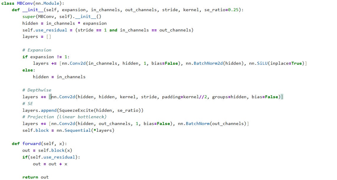
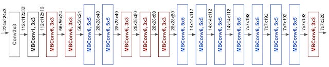
Building Block: MBConv

An MBConv block combines three ideas:

1. Inverted residual block (from MobileNetV2)

2. Depthwise separable convolution

3. Squeeze-and-Excitation (SE) attention (from MobileNetV3)

Structure

1. 1×1 expansion conv (increase channels)

2. Depthwise 3×3 or 5×5 conv

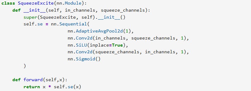
3. Squeeze-and-Excitation (SE)

   • Channel-wise attention:

     • Global Avg Pool → FC → FC → sigmoid

     • Reweights channels adaptively

4. 1×1 projection conv

5. Skip connection (if stride = 1)

From [3], Starting from Baseline EfficientNet-B0, compound scaling method to scale up is as follows

• Fix ϕ = 1, Best values for the baseline, α = 1.2, β = 1.1 , γ = 1.15

• Now fix α, β, γ as constants and scale up the baseline network with different ϕ using the equation mentioned before, to obtain EfficientNet-B1 to B7

Fig.4: Architecture for EfficientNet-B0[7]

Practical Insights

1. Parameter counts are highly sensitive to architectural details

   • Although EfficientNet-B0 is commonly reported to have ~5.3M parameters, small implementation choices can easily shift this number by millions

2. Squeeze-and-Excitation bottleneck sizing is critical

   • common mistake: computing the SE bottleneck from the expanded channel dimension of MBConv blocks.

   • In EfficientNet, the SE bottleneck is instead computed from the input channels of the block, even though SE is applied to the expanded feature map.

   • Formally:

     • Expanded channels = C_in​ × t

     • SE bottleneck = C_in // 4

3. Bias terms in SE layers affect parameter count. Torchvision’s EfficientNet includes bias terms in SE convolutions. Removing these biases reduces parameter count but creates a leaner variant rather than an exact reproduction of the reference implementation.

   

Closing Thoughts

DenseNet, MobileNet, and EfficientNet approach efficiency from very different directions—feature reuse, computation reduction, and principled scaling. Small deviations in block configuration or scaling logic can significantly impact parameter count and performance.

In particular, EfficientNet demonstrates that architectural discipline matters as much as architectural novelty. Subtle details such as squeeze-and-excitation bottleneck sizing, head width, and normalization placement can change parameter counts by millions and significantly alter efficiency.

References

[1] Densely Connected Convolutional Networks

[2] MobileNets: Efficient Convolutional Neural Networks for Mobile Vision Applications

[3] EfficientNet: Rethinking Model Scaling for Convolutional Neural Networks

[4] MobileNetV2: Inverted Residuals and Linear Bottlenecks

[5] Searching for MobileNetV3

[6] Squeeze-and-Excitation Networks

[7] Google Blog on EfficientNet

[8] Pytorch EfficientNet implementation